Experiment 2

Author

Yuan

Published

April 21, 2023

Modified

May 20, 2023

更新日志

2023-4-26: 修改第七题

写在前面

介绍

同学们好，以下是中级计量经济学第二次实验的参考，完全由本人制作。其中除了第一题以外，涉及统计学、计量经济学知识的部分，由于本人水平有限，无法保证完全正确。仅供同学们学习参考。如果你有任何问题或者发现了哪里有错，可以在右边用Hypothesis标注并评论，与大家一同讨论，或者私下联系我。我会在看到的第一时间回复你的！

感受

写完一遍这次实验下来，感觉还是收获颇多。还是有很多细节需要多多琢磨，从R语言，到统计学、计量经济学的知识，不管是假设检验部分，logit/probit 部分，TSLS部分，还是作图、做表方面都有很多考究，日后还是要多多研究。希望同学们可以抱着多多学习交流，认真仔细钻研每道题的心态来做这次的实验内容。

关于需要耗费的时间。如果是单纯分析问题，可能2-7题每道题需要两个小时左右，加上思考代码结构、思考如何作图作表，我个人花了两周的时间（几乎每天的主要精力都在研究本次实验），在无聊时拿起来想一想这些问题，也是趣味颇多的一件事情（相比于我的室友那令人痛苦的信号与系统云云，我觉得思考计量问题还是挺怡然自得的）。

日后我还会对内容稍加修改，包括纠错、增加讲解之类的。还是那句话，希望同学们多多交流！

导入依赖包

# input libraries
library(gmodels)
library(officedown)
library(car)
library(dplyr)
library(ggplot2)
library(readxl)
library(flextable)
library(stats4)
library(plm)
library(patchwork)
library(sjPlot)
library(AER)
library(magrittr)
library(infer)

Problem 1(Likelihood Function)

Data Read and Manipulation

The xlsx data can be read with readxl library. Then it is convert to matrix, split by x and y,

hmda <- read_xlsx("data/hmda_sw.xlsx")
hmda <- hmda %>%
  mutate(
    black = ifelse(s13 == 3, 1, 0),
    deny = ifelse(s7 == 3, 1, 0),
    PI = s46 / 100,
    hse_inc = s45 / 100,
    loan_val = s6 / s50,
    ccred = s43,
    mcred = s42,
    pubrec = 1 * (s44 > 0),
    denpmi = 1 * (s53 == 1),
    selfemp = 1 * (s27a == 1),
    married = 1 * (s23a == "M"),
    single = 1 * (married == 0),
    hischl = 1 * (school >= 12),
    probunmp = uria,
    condo = 1 * (s51 == 1)
  )

#   deop the unused colomns
hmda <- hmda %>%
  select(
    black, deny, PI, hse_inc,
    loan_val, ccred, mcred, pubrec,
    denpmi, selfemp, married, single,
    hischl, probunmp, condo
  )

Gene rate loan-to-value ration with 3 levels(high if loan_val > 0.95, low if loan_val < 0.8, medium otherwise)

hmda <- hmda %>%
  mutate(
    lvratmedium = ifelse(loan_val >= 0.8 & loan_val <= 0.95, 1, 0),
    lvrathigh = ifelse(loan_val > 0.95, 1, 0)
  )

OLS Estimator

attach(hmda)
mod.deny <- lm(
  deny ~ 1 + black + PI + hse_inc + lvratmedium + lvrathigh +
    ccred + mcred + pubrec + denpmi + selfemp
)
detach(hmda)
coef <- mod.deny$coefficients
coef_from_textbook <- c(
  -0.183, 0.084, 0.449, -0.048, 0.031, 0.189, 0.031,
  0.021, 0.197, 0.702, 0.060
)
coef_comp <- tibble(name = names(coef), coef = coef, coef_book = coef_from_textbook) %>%
  mutate(coef = round(coef, 3))
coef_comp %>%
  flextable() %>%
  align(part = "header", align = "center") %>%
  bold(part = "header") %>%
  autofit()

Table 1:
HMDA coefficients of OLS comparison
name	coef	coef_book
(Intercept)	-0.183	-0.183
black	0.084	0.084
PI	0.449	0.449
hse_inc	-0.048	-0.048
lvratmedium	0.031	0.031
lvrathigh	0.189	0.189
ccred	0.031	0.031
mcred	0.021	0.021
pubrec	0.197	0.197
denpmi	0.702	0.702
selfemp	0.060	0.060

The coefficients of above OLS regression result are same comparing to the table 11.2 on textbook.

Probit Model

Likelihood Function

Develop the likelihood function of MLE, following the textbook Ch11. Because there is only \(Y_1\), The likelihood function will be

\[ f(\beta_0,\beta_1,...,\beta_n;Y_1,...,Y_{m}|X_1,...,X_m) \]

\[ =\{\Theta(\beta_0+\beta_1X_{11}+...+\beta_nX_{1n})^{Y_1}[1-\Theta(\beta_0+\beta_1X_{11}+\beta_nX_{1n})]^{1-Y_1} \}\times \]

\[ ...\times \{\Theta(\beta_0+\beta_1X_{m1}+...+\beta_nX_{mn})^{Y_m}[1-\Theta(\beta_0+\beta_1X_{m1}+...+\beta_nX_{mn})]^{1-Y_m}\} \]

Where \(\hat{\beta}_0^{MLE}, ..., \hat{\beta}_n^{MLE}\) maximize this likelihood function.

Logarithm of the likelihood:

\[ ln(f(\beta_0,\beta_1,\beta_n;Y_1,...,Y_{m}|X_1,...,X_m)) \]

\[ = Y_1ln(\Theta( \beta_0+\beta_1X_{11}+...+\beta_nX_{1n}))+(1-Y_1)ln (1-\Theta(\beta_0+\beta_1X_{11}+\beta_nX_{1n}))+ \]

\[ ...+ Y_mln(\Theta(\beta_0+\beta_1X_{m1}+...+\beta_nX_{mn}))+ (1-Y_m)ln(1-\Theta(\beta_0+\beta_1X_{m1}+...+\beta_nX_{mn})) \]

# x is a matrix with n * n
# y is a matrix with n * 1
# beta is the vector to maximize
likefunc_probit <- function(beta, x, y) {
  x <- cbind(1, x)
  res <- 0
  beta <- c(beta)
  for (i in 1:nrow(x)) {
    theta <- pnorm(x[i, ] %*% beta)
    res <- res +
      y[i, ] * log(theta) +
      (1 - y[i, ]) * log(1 - theta)
  }
  return(-res)
}

Beta Generation and Comparison

#| warning: false
#| message: false
attach(hmda)
x <- hmda %>%
  select(
    black, PI, hse_inc, lvratmedium, lvrathigh,
    ccred, mcred, pubrec, denpmi, selfemp
  ) %>%
  as.matrix()
y <- hmda %>%
  select(deny) %>%
  as.matrix()
detach(hmda)

res_probit <- optim(rep(0, 11),
  likefunc_probit,
  x = x, y = y, method = "BFGS"
)
res_probit_book <- c(
  -3.04, 0.389, 2.44, -0.18, 0.21, 0.79,
  0.15, 0.15, 0.7, 2.56, 0.36
)

Table 2:
HMDA probit model results comparison
Name	Probit Implemented	Result from Textbook
(Intercept)	-3.041	-3.040
black	0.389	0.389
PI	2.442	2.440
hse_inc	-0.185	-0.180
lvratmedium	0.214	0.210
lvrathigh	0.791	0.790
ccred	0.155	0.150
mcred	0.148	0.150
pubrec	0.697	0.700
denpmi	2.557	2.560
selfemp	0.359	0.360

Logit Model

Likelihood Function

The difference between Logit and Probit model is the cumulative distribution function. The CDF of Logit model is

\[ F(\beta_0+\beta_1X_1+...+\beta_nX_n)=\frac{1}{1+e^{-(\beta_0+\beta_1X_1+...+\beta_nX_n)}} \]

So the likelihood function is

\[ f(\beta_0,\beta_1,...,\beta_n;Y_1,...,Y_{m}|X_1,...,X_m) \]

\[ =\{F(\beta_0+\beta_1X_{11}+...+\beta_nX_{1n})^{Y_1}[1-F(\beta_0+\beta_1X_{11}+\beta_nX_{1n})]^{1-Y_1} \}\times \]

\[ ...\times \{F(\beta_0+\beta_1X_{m1}+...+\beta_nX_{mn})^{Y_m}[1-F(\beta_0+\beta_1X_{m1}+...+\beta_nX_{mn})]^{1-Y_m}\} \]

the log form is:

\[ ln(f(\beta_0,\beta_1,\beta_n;Y_1,...,Y_{m}|X_1,...,X_m)) \]

\[ = Y_1ln(F( \beta_0+\beta_1X_{11}+...+\beta_nX_{1n}))+(1-Y_1)ln (1-F(\beta_0+\beta_1X_{11}+\beta_nX_{1n}))+ \]

\[ ...+ Y_mln(F(\beta_0+\beta_1X_{m1}+...+\beta_nX_{mn}))+ (1-Y_m)ln(1-F(\beta_0+\beta_1X_{m1}+...+\beta_nX_{mn})) \]

Implement it in r:

# x is a matrix with n * n
# y is a matrix with n * 1
# beta is the vector to maximize
logit <- function(x) {
  res <- 1 / (1 + exp(-x))
  return(res)
}

likefunc_logit <- function(beta, x, y) {
  x <- cbind(1, x)
  res <- 0
  beta <- c(beta)
  for (i in 1:nrow(x)) {
    f <- logit(x[i, ] %*% beta)
    res <- res +
      y[i, ] * log(f) +
      (1 - y[i, ]) * log(1 - f)
  }
  return(-res)
}

Beta Generation and Comparison

res_logit <- optim(rep(0, 11), likefunc_logit, x = x, y = y, method = "BFGS")
res_logit_book <- c(-5.71, 0.688, 4.76, -0.11, 0.46, 1.49, 0.29, 0.28, 1.23, 4.55, 0.67)

Table 3:
HMDA logit model results comparison
Name	Logit Implemented	Result From Book
(Intercept)	-5.707	-5.710
black	0.688	0.688
PI	4.764	4.760
hse_inc	-0.109	-0.110
lvratmedium	0.464	0.460
lvrathigh	1.495	1.490
ccred	0.290	0.290
mcred	0.279	0.280
pubrec	1.226	1.230
denpmi	4.548	4.550
selfemp	0.666	0.670

The above comparisons show that the likelihood functions are developed, and coefficients are estimated, successfully.

Problem 2(Seatbelts)

a.

seatbelts <- read_xls("data/SeatBelts.xls")
attach(seatbelts)
mod.seat1 <- lm(
  fatalityrate ~ 1 + sb_useage + speed65 + speed70 + ba08 + drinkage21 + log(income) + age
)
detach(seatbelts)

From the regression, increased seat belt use enlarges fatalities.

b.

Compare the coefficients between two models. The coefficient of sb_useage changed from positive to negative. There may be some properties of states caused the bias. After fixing state, it becomes more reasonable.

c.

After adding time fixed effects plus state fixed effects, the coefficient of sb_useage is still negative when fixing state and year, which indicates that higher seat belt use rate reduces fatalities.

attach(seatbelts)
mod.seat3 <- seatbelts %>% plm(
  fatalityrate ~ sb_useage + speed65 + speed70 + ba08 + drinkage21 + log(income) + age,
  effect = "twoway",
  index = c("state", "year"),
  data = .
)
detach(seatbelts)

Table 4: Coef.: no fixing, fix state, fix state plus year
	without fixing	fix state	fix state plus year
Predictors	Estimates	Estimates	Estimates
(Intercept)	0.1965 ^*** (0.0082)
sb_useage	0.0041 ^*** (0.0012)	-0.0058 ^*** (0.0012)	-0.0037 ^** (0.0011)
speed65	0.0001 (0.0004)	-0.0004 (0.0003)	-0.0008 (0.0004)
speed70	0.0024 ^*** (0.0005)	0.0012 ^*** (0.0003)	0.0008 ^* (0.0003)
ba08	-0.0019 ^*** (0.0004)	-0.0014 ^*** (0.0004)	-0.0008 ^* (0.0004)
drinkage21	0.0001 (0.0009)	0.0007 (0.0005)	-0.0011 ^* (0.0005)
log(income)	-0.0181 ^*** (0.0009)	-0.0135 ^*** (0.0014)	0.0063 (0.0039)
age	-0.0000 (0.0001)	0.0010 ^* (0.0004)	0.0013 ^*** (0.0004)
Observations	556	556	556
R² / R² adjusted	0.549 / 0.544	0.687 / 0.651	0.083 / -0.052
* p<0.05 p<0.01 * p<0.001

d.

Regression in (c), with state and year fixed is most reliable. Because it fixes the effects of different years and states, of which the coefficient of sb_useage is most precise.

e.

Th e coefficient of sb_useage is -0.0037, indicating that with 1% seat belt use increased, fatalities will reduce by 0.37%. It is a large number. It means that if seat belt use increase from 52% to 90%, about 58 lives will be saved(counted by average millions of traffic miles per year).

f.

attach(seatbelts)
mod.seat4 <- seatbelts %>% plm(
  sb_useage ~ primary + secondary + speed65 + speed70 + ba08 + drinkage21 + log(income) + age,
  data = .,
  index = c("state", "year"),
  effect = "twoway"
)
detach(seatbelts)

Table 5: Primary and Secondary, Fixed Years and States
	sb_useage
Predictors	Estimates	std. Error	CI
primary	0.2056 ^***	0.0281	0.1503 – 0.2609
secondary	0.1085 ^***	0.0104	0.0880 – 0.1290
speed65	0.0228	0.0153	-0.0071 – 0.0528
speed70	0.0120	0.0121	-0.0116 – 0.0357
ba08	0.0038	0.0125	-0.0208 – 0.0283
drinkage21	0.0107	0.0197	-0.0280 – 0.0494
log(income)	0.0583	0.1372	-0.2114 – 0.3279
age	0.0138	0.0136	-0.0129 – 0.0406
Observations	556
R² / R² adjusted	0.249 / 0.138
* p<0.05 p<0.01 * p<0.001

The regression result shows that primary enforcement leads to more seat belt use. Secondary enforcement, too, leads to more seat belt use.

g.

\[ sub\space useage=0.206\times primary+0.109\times secondary+... \]

New Jersey changed from secondary enforcement to primary enforcement, which means:

\[ primary: 0 \rightarrow1, secondary:1\rightarrow0 \]

\[ \Delta sb \space useage=0.206-0.109=0.097 \]

This is predicted to reduce the fatality rate by \(0.00372\times 0.097=0.00036\) fatalities per million traffic mile.

\[ \Delta fatality\space rate=-0.00372\times \Delta sb\space useage=0.00372\times 0.097=0.00036 \]

The data set shows that there were 6300 million traffic miles in 1997 in New Jersey. Assuming that same number of traffic miles in 2000 yields \(0.00036\times 63,000=23\) lives saved.

Problem 3(JEC)

a.

The model is

\[ ln(Q_i)=\beta_0+\beta_1ln(P_i)+\beta_2Ice_i+\Sigma^{12}_{j=1}\beta Seas_{j,i}+u_i \]

jec <- read_xls("data/JEC.xls")

attach(jec)
mod.jec1 <- lm(
  log(quantity) ~ 1 + log(price) + ice + seas1 + seas2 + seas3 + seas4 +
    seas5 + seas6 + seas7 + seas8 + seas9 + seas10 + seas11 + seas12
)
detach(jec)

The regression result shows that the demand elasticity is -0.639 and its standard error is 0.082

b.

There is simultaneous causality in the interaction of supply and demand, thus it makes the OLS estimator of the elasticity biased.

c.

The collusion of the cartel increases the price of grain what would have been the competitive price, i.e. \(Corr(cartel, ln(price))>0\). But the cartel and change price do not influence the demand of grain, for grain is necessary, which means \(Corr(cartel, ln(Q))=0\). The two correlations above illustrate that cartel is a valid instrument.

d.

Model of Stage 1:

\[ ln(P_i)=\beta_0+\beta_1 cartel+\beta_2Ice_i+\Sigma^{12}_{j=1}\beta Seas_{j,i}+u_i \]

attach(jec)
mod.jec_stage1 <- lm(
  log(price) ~ 1 + cartel + ice + seas1 + seas2 + seas3 + seas4 +
    seas5 + seas6 + seas7 + seas8 + seas9 + seas10 + seas11 + seas12
)
detach(jec)

The first state F-statistic, 21.3170209, which is > 10, illustrates that the estimators in first stage are jointly significant. That means cartel is not a weak instrument.

e.

The model of second stage:

\[ ln(Q_i)=\beta_0+\beta_1\widehat{ln(P_i)}+\beta_2Ice_i+\Sigma^{12}_{j=1}\beta Seas_{j,i}+w_i \]

pred_logp <- fitted.values(mod.jec_stage1)
attach(jec)
mod.jec_stage2 <- ivreg(
  log(quantity) ~ 1 + log(price) + ice + seas1 + seas2 + seas3 + seas4 +
    seas5 + seas6 + seas7 + seas8 + seas9 + seas10 + seas11 + seas12 |
    cartel + ice + seas1 + seas2 + seas3 + seas4 +
      seas5 + seas6 + seas7 + seas8 + seas9 + seas10 + seas11 + seas12
)
detach(jec)

The regression result shows that estimated demand elasticity is -0.867 and its standard error is 0.132.

Table 6: JEC Regression Results(FE on Seasons)
	Elasticity	TSLS stage 1	TSLS stage 2
Predictors	Estimates	Estimates	Estimates
(Intercept)	8.8612 ^*** (0.1714)	-1.6937 ^*** (0.0784)	8.5735 ^*** (0.2164)
price [log]	-0.6389 ^*** (0.0824)		-0.8666 ^*** (0.1321)
cartel		0.3579 ^*** (0.0249)
Observations	328	328	328
R² / R² adjusted	0.313 / 0.282	0.488 / 0.465	0.296 / 0.264
* p<0.05 p<0.01 * p<0.001

f.

The absolute price elasticity is less than 1, so marginal profit is positive, which prompts the cartel to raise the price. So it suggests that the cartel was charging the profit-maximizing monopoly price.

Problem 4(Movies)

a.

i.

movies <- read_xlsx("data/Movies.xlsx")

The Model is as follows:

\[ log(assaults_i) = \beta_0 + \Sigma^{10}_{j=2}\beta year_{j,i}+\Sigma^{12}_{j=2}\beta month_{j,i} + u_i \]

Choose year1, month1 as the basic group, to avoid the dummy variable trap. Then regress log(assaults) on years and months

attach(movies)
mod.movies1 <- lm(
  log(assaults) ~ 1 + year2 + year3 + year4 + year5 + year6 + year7 + year8 + year9 +
    year10 + month2 + month3 + month4 + month5 + month6 + month7 + month8 + month9 +
    month10 + month11 + month12
)
detach(movies)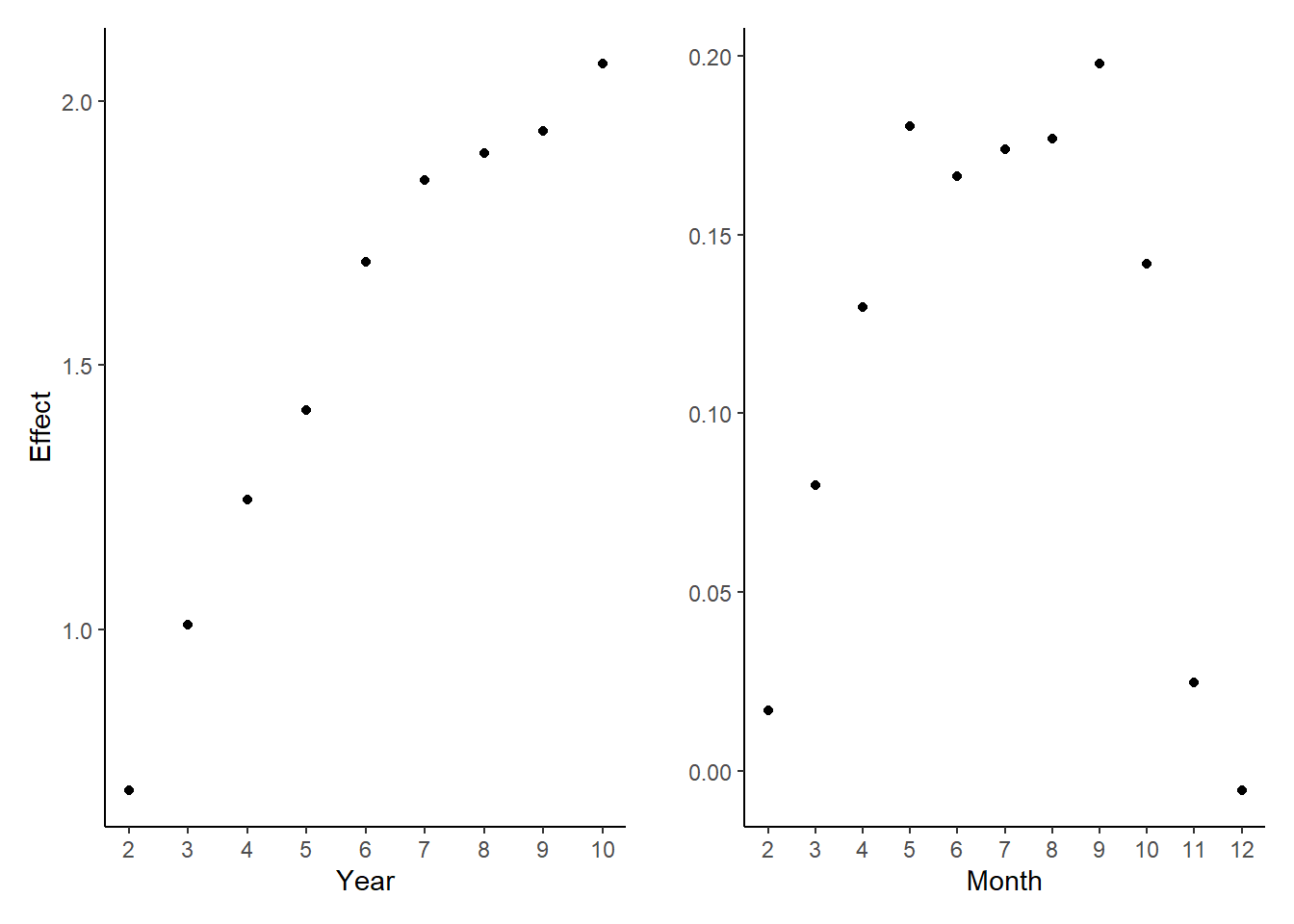

Figure 1: Reg assault: Effects of Years and Months on Assaults

mod.movies1_f <- mod.movies1 %>%
  linearHypothesis(c(
    "month2=month3",
    "month2=month4",
    "month2=month5",
    "month2=month6",
    "month2=month7",
    "month2=month8",
    "month2=month9",
    "month2=month10",
    "month2=month11",
    "month2=month12"
  )) %>%
  .["F"] %>%
  pull() %>%
  .[2] %>%
  round()

The regression result shows that assaults increases with year. And there are more assaults in month 5-10, less in month 1, 12. And the F-statistic on the 11 monthly indicators is 67 with p-value that is essentially 0. So the seasonality in assaults exists.

ii.

# Generate attend
movies <- movies %>% mutate(attend = attend_v + attend_m + attend_n)
attach(movies)
mod.attend1 <- lm(
  attend ~ 1 + year2 + year3 + year4 + year5 + year6 + year7 + year8 + year9 +
    year10 + month2 + month3 + month4 + month5 + month6 + month7 + month8 + month9 +
    month10 + month11 + month12
)
detach(movies)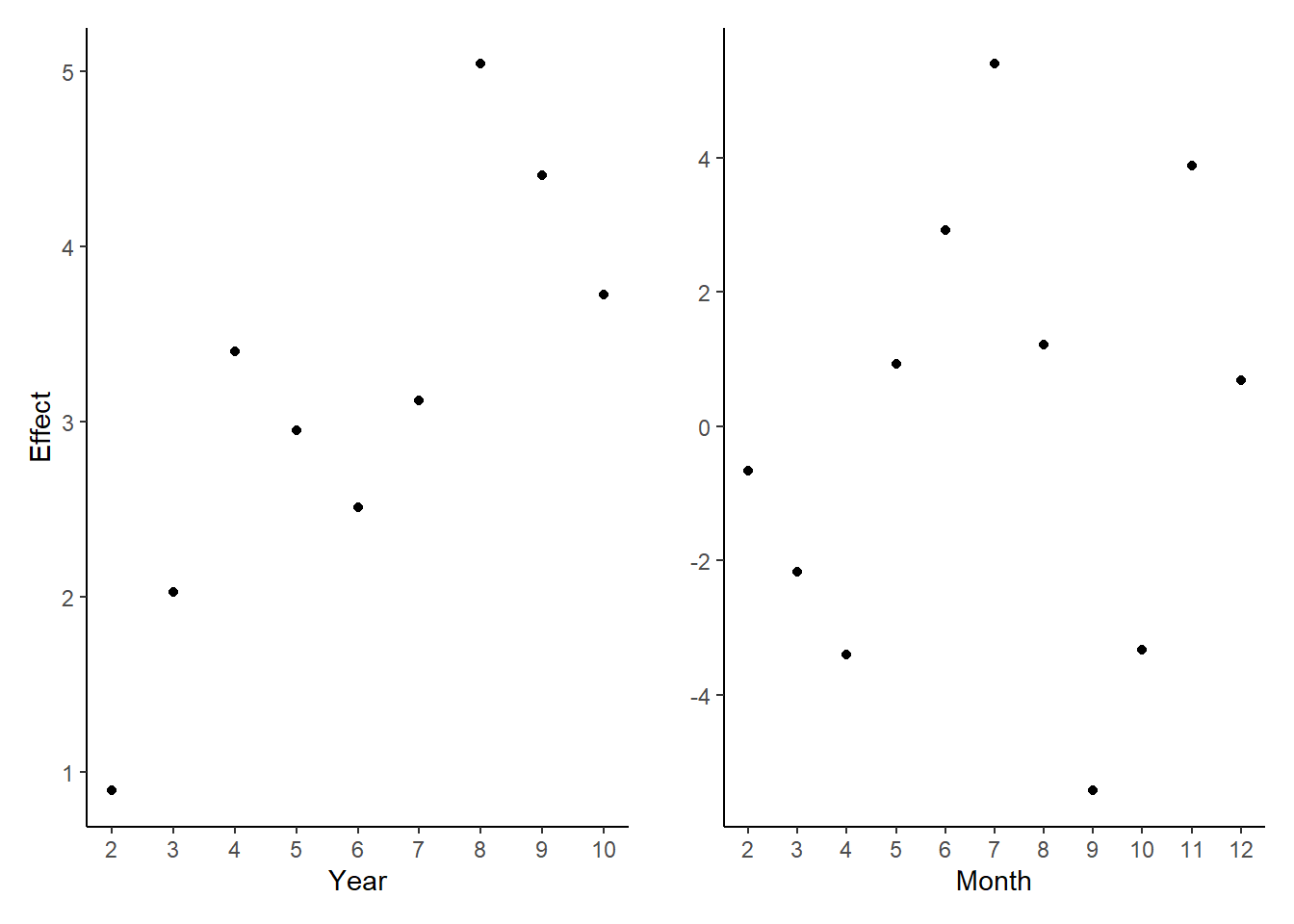

Figure 2: Reg attend: Effects of Years and Months on Movie Attend

attend_months_f <- mod.attend1 %>%
  linearHypothesis(c(
    "month2=month3",
    "month2=month4",
    "month2=month5",
    "month2=month6",
    "month2=month7",
    "month2=month8",
    "month2=month9",
    "month2=month10",
    "month2=month11",
    "month2=month12"
  )) %>%
  .["F"] %>%
  pull() %>%
  .[2] %>%
  round()

From the figure, the difference of the coefficient among years is significant. The difference among months is significant, too. And the F-statistic on the 11 monthly indicators is 37 with p-value that is essentially 0. So there is seasonality in movie attendance.

b.

i.

attach(movies)
mod.ln_ass <- lm(
  log(assaults) ~ 1 + attend_v + attend_m + attend_n + year2 + year3 + year4 +
    year5 + year6 + year7 + year8 + year9 + year10 + month2 + month3 + month4 +
    month5 + month6 + month7 + month8 + month9 + month10 + month11 + month12 +
    h_chris + h_newyr + h_easter + h_july4 + h_mem + h_labor +
    w_rain + w_snow + w_maxa + w_maxb + w_maxc + w_mina + w_minb + w_minc
)
detach(movies)

Table 7:
Regress ln_assaults on v, n, m, year, month, weather, and holidy
Var.Name	Estimate	Std. Error	t value	Pr(>\|t\|)
(Intercept)	6.91432	0.01715	403.24547	0.00000
attend_v	-0.00317	0.00100	-3.17102	0.00162
attend_m	-0.00314	0.00066	-4.74238	0.00000
attend_n	-0.00211	0.00066	-3.19400	0.00150
Note. Fixed variables are hidden

The regression result shows that viewing a strongly violent movie decreases assaults by 0.32%. The estimated effect is statistically significant at 0.01 significant level.

ii.

Make hypothesis that \(\beta_v = \beta_m\) and \(\beta_v = \beta_n\). Then do F tests.

Table 8:
F test of v=m, v=n
Test	F	Pr(>F)
v=m	0.00113	0.97325
v=n	1.21960	0.27000

The F-test result suggests that \(\beta_v\) with \(\beta_m\), and \(beta_v\) with \(\beta_n\) have no statistically significant difference from one another.

iii.

Construct a new variable effect and construct its 95% confidence interval.

\[ effect = 6*\beta_v * attend_v-2*\beta_m*attend_m-\beta_n*attend_n \]

beta_v <- mod.ln_ass$coefficients["attend_v"]
beta_m <- mod.ln_ass$coefficients["attend_m"]
beta_n <- mod.ln_ass$coefficients["attend_n"]
effect <- movies %>%
  mutate(effect = 6 * beta_v * attend_v -
    2 * beta_m * attend_m -
    beta_n * attend_n) %>%
  select(effect) %>%
  pull()
ci_res <- ci(effect) %>%
  as.data.frame() %>%
  t() %>%
  as.data.frame() %>%
  round(5)

The OLS estimate for this coefficient is 0.01553. It shows a decrease in assaults of 1.55%. The 95% confidence interval is (0.01056, 0.02051).

Table 9:
Confidence Interval of Prediction
Estimate	CI lower	CI upper	Std. Error
0.01553	0.01056	0.02051	0.00253

c.

Use pr_attend_v, pr_attend_m, and pr_attend_n as instruments for attend_v, attend_m, and attend_n. Run the regression.

mod.movies_tsls <- ivreg(
  data = movies,
  log(assaults) ~ attend_v + attend_m + attend_n + year2 + year3 + year4 +
    year5 + year6 + year7 + year8 + year9 + year10 + month2 + month3 + month4 +
    month5 + month6 + month7 + month8 + month9 + month10 + month11 + month12 +
    h_chris + h_newyr + h_easter + h_july4 + h_mem + h_labor +
    w_rain + w_snow + w_maxa + w_maxb + w_maxc + w_mina + w_minb + w_minc |
    pr_attend_v + pr_attend_m + pr_attend_n + year2 + year3 + year4 +
      year5 + year6 + year7 + year8 + year9 + year10 + month2 + month3 + month4 +
      month5 + month6 + month7 + month8 + month9 + month10 + month11 + month12 +
      h_chris + h_newyr + h_easter + h_july4 + h_mem + h_labor +
      w_rain + w_snow + w_maxa + w_maxb + w_maxc + w_mina + w_minb + w_minc
)

Table 10:
Movies TSLS Stage 2 Result
Var.Name	Estimate	Std. Error	t value	Pr(>\|t\|)
(Intercept)	6.92418	0.01828	378.83439	0.00000
attend_v	-0.00387	0.00111	-3.48016	0.00055
attend_m	-0.00389	0.00077	-5.02473	0.00000
attend_n	-0.00272	0.00079	-3.44928	0.00061
Note. Fixed variables are hidden

So based on this regression, viewing strongly violent movies leads to a small but significant decrease in assaults, rather than an increase.

Samely, make the linear hypothesis attend_v=attend_m and attend_v=attend_n

movies_tsls_vm <- mod.movies_tsls %>% car::linearHypothesis(
  "attend_v=attend_m"
)
movies_tsls_vn <- mod.movies_tsls %>% car::linearHypothesis(
  "attend_v = attend_n"
)

Table 11:
TSLS F test of v=m, v=n
Test	Chisq	Pr(>Chisq)
v=m	0.00041	0.98377
v=n	1.34368	0.24639

Too, the F-test result suggests that \(\beta_v\), \(\beta_m\), \(\beta_n\) have no statistically significant difference from one another.

beta_v <- mod.movies_tsls$coefficients["attend_v"]
beta_m <- mod.movies_tsls$coefficients["attend_m"]
beta_n <- mod.movies_tsls$coefficients["attend_n"]
effect <- movies %>%
  mutate(effect = 6 * beta_v * attend_v -
    2 * beta_m * attend_m -
    beta_n * attend_n) %>%
  select(effect) %>%
  pull()
ci_res_tsls <- ci(effect) %>%
  as.data.frame() %>%
  t() %>%
  as.data.frame() %>%
  round(5)

The OLS estimate for this coefficient is 0.02115. It shows a decrease in assaults of 2.11%. The 95% confidence interval is (0.01503, 0.02726).

Table 12:
Change in Assaults 95% Confidence Interval
Estimate	CI lower	CI upper	Std. Error
0.02115	0.01503	0.02726	0.00311

d.

attend_v_f, attend_m_f, attend_n_f, attend_v_b, attend_m_b, and attend_n_b

mod.movies_tsls2 <- ivreg(
  data = movies,
  log(assaults) ~ attend_v + attend_m + attend_n + year2 + year3 + year4 +
    year5 + year6 + year7 + year8 + year9 + year10 + month2 + month3 + month4 +
    month5 + month6 + month7 + month8 + month9 + month10 + month11 + month12 +
    h_chris + h_newyr + h_easter + h_july4 + h_mem + h_labor +
    w_rain + w_snow + w_maxa + w_maxb + w_maxc + w_mina + w_minb + w_minc |
    attend_v_f + attend_m_f + attend_n_f + attend_v_b + attend_m_b + attend_n_b + year2 + year3 + year4 +
      year5 + year6 + year7 + year8 + year9 + year10 + month2 + month3 + month4 +
      month5 + month6 + month7 + month8 + month9 + month10 + month11 + month12 +
      h_chris + h_newyr + h_easter + h_july4 + h_mem + h_labor +
      w_rain + w_snow + w_maxa + w_maxb + w_maxc + w_mina + w_minb + w_minc
)

Table 13:
Movies TSLS(2) Stage 2 Result
Var.Name	Estimate	Std. Error	t value	Pr(>\|t\|)
(Intercept)	6.92252	0.02644	261.85541	0.00000
attend_v	-0.00317	0.00205	-1.54546	0.12290
attend_m	-0.00412	0.00151	-2.72450	0.00668
attend_n	-0.00258	0.00154	-1.67705	0.09419
Note. Fixed variables are hidden

movies_tsls_vm <- mod.movies_tsls2 %>% car::linearHypothesis(
  "attend_v=attend_m"
)
movies_tsls_vn <- mod.movies_tsls2 %>% car::linearHypothesis(
  "attend_v = attend_n"
)

Table 14:
TSLS F test of v=m, v=n
Test	Chisq	Pr(>Chisq)
v=m	0.37994	0.53763
v=n	0.17518	0.67555

beta_v <- mod.movies_tsls2$coefficients["attend_v"]
beta_m <- mod.movies_tsls2$coefficients["attend_m"]
beta_n <- mod.movies_tsls2$coefficients["attend_n"]
effect <- movies %>%
  mutate(effect = 6 * beta_v * attend_v -
    2 * beta_m * attend_m -
    beta_n * attend_n) %>%
  select(effect) %>%
  pull()
ci_res_tsls2 <- ci(effect) %>%
  as.data.frame() %>%
  t() %>%
  as.data.frame() %>%
  round(5)

Table 15:
Change in Assaults 95% Confidence Interval
Estimate	CI lower	CI upper	Std. Error
0.03412	0.02863	0.03961	0.0028

The results are same comparing to b, or c.

e.

Use J-test to test the overidentifying restrictions

# TSLS 
model <- ivreg(log(assaults) ~ attend_v + attend_m + attend_n + year2 + year3 + year4 +
    year5 + year6 + year7 + year8 + year9 + year10 + month2 + month3 + month4 +
    month5 + month6 + month7 + month8 + month9 + month10 + month11 + month12 +
    h_chris + h_newyr + h_easter + h_july4 + h_mem + h_labor +
    w_rain + w_snow + w_maxa + w_maxb + w_maxc + w_mina + w_minb + w_minc | 
      pr_attend_v + pr_attend_m + pr_attend_n + attend_v_f + attend_m_f + 
      attend_n_f + attend_v_b + attend_m_b + attend_n_b + year2 + year3 + year4 +
      year5 + year6 + year7 + year8 + year9 + year10 + month2 + month3 + month4 +
      month5 + month6 + month7 + month8 + month9 + month10 + month11 + month12 +
      h_chris + h_newyr + h_easter + h_july4 + h_mem + h_labor +
      w_rain + w_snow + w_maxa + w_maxb + w_maxc + w_mina + w_minb + w_minc, 
      data = movies)

# Predicted values 
y_hat <- predict(model)

# Residuals
u_hat <- log(movies$assaults) - y_hat

# Regress residuals on instruments and exog. vars
resid_model <- lm(
  u_hat ~ pr_attend_v + pr_attend_m + pr_attend_n + attend_v_f + attend_m_f + 
      attend_n_f + attend_v_b + attend_m_b + attend_n_b + year2 + year3 + year4 +
      year5 + year6 + year7 + year8 + year9 + year10 + month2 + month3 + month4 +
      month5 + month6 + month7 + month8 + month9 + month10 + month11 + month12 +
      h_chris + h_newyr + h_easter + h_july4 + h_mem + h_labor +
      w_rain + w_snow + w_maxa + w_maxb + w_maxc + w_mina + w_minb + w_minc, data = movies
)  

# F-statistic
f_stat <- resid_model %>% car::linearHypothesis(
  c("pr_attend_v=0",
  "pr_attend_v=pr_attend_m",
  "pr_attend_m=pr_attend_n",
  "pr_attend_n=attend_v_f",
  "attend_v_f=attend_m_f",
  "attend_m_f=attend_n_f",
  "attend_n_f=attend_v_b",
  "attend_v_b=attend_m_b",
  "attend_m_b=attend_n_b")
) %>% .["F"] %>% pull() %>% .[2]

# J-statistic 
j_stat <- 9 * f_stat

The J-stat is 8.5937298. We failed to reject the hypothesis that all instruments are exogenous, which means that some of the instruments are invalid.

f.

The violent movies won’t affect, or will slightly decrease violent behavior.

Problem 5(Fertility)

fertility <- read_xlsx("data/fertility.xlsx")

a.

attach(fertility)
mod.fertility1 <- lm(
  weeksm1 ~ 1 + morekids
)
detach(fertility)

The regression result suggests that women with more than two children work about 5 weeks less than women with two children.

b.

Selection bias: The sample only includes married women who already have at least 2 children. Women who never married or had children may have different effects, so the estimates cannot be generalized.
Simultaneous causality: Labor supply may also affect fertility decisions, not just the other way around. So weeksworked should also be treated as endogenous.
Omitted variable bias: There may be omitted factors that affect both fertility and labor supply, such as religion, education, career ambition, etc. If these are not controlled for, the OLS estimates will be biased.

c.

mod.morekids_on_samesex <- glm(
  morekids ~ samesex,
  family = binomial(link = "logit"),
  data = fertility
)

To predict the effect of same sex of first two children on the third child, run a logit model of morekids on samesex, the regression result shows:

\[ Probit(morekids) = -0.635+0.287*samesex \]

The marginal effect of samesex is \(0.287*(\phi(-0.635+0.287))=0.107\). When samesex increases from 0 to 1, the probability increases by 10.7%. This appears to be a reasonably large and meaningful effect, indicating having same-sex first two children meaningfully impacts the probability of having a third child. From the p-value of the regression result, the coefficient is statistically significant.

d.

Relevance: samesex is correlated with morekids. Discussion in c. has proved that having same-sex first two children is positive correlated with more kids. So samesex satisfies the relevance criterion for an IV.
Exogeneity: samesex is unlikely to directly affect weeksworked. Whether the first two children are the same gender is exogenous to the mother’s labor supply. So samesex satisfies the exogeneity assumption.

e.

In the first stage, F-stat is 1237>10, so it is not a weak instrument.

f.

# stage 1
mod.fertility_stage1 <- lm(
  morekids ~ samesex,
  data = fertility
)
# stage 2
mod.fertility_stage2 <- ivreg(
  weeksm1 ~ 1 + morekids | samesex,
  data = fertility
)

From the TSLS, more than two kids decreases about -6.3 working weeks.

g.

After including the variables agem1, black, hispan, and othrace in the labor supply regression, the effect of more kids is still negative, but shrink a little to 0, which is now -5.8. This is because morekids indeed has negative effect on labor supply, but after including fixed effect, the missing-variable bias is basically eliminated.

# stage 1 with FE
mod.fertility_stage1_fixed <- glm(
  morekids ~ samesex + agem1 + black + hispan + othrace,
  family = binomial(link = "logit"),
  data = fertility
)
# stage 2 with FE
mod.fertility_stage2_fixed <- ivreg(
  data = fertility,
  weeksm1 ~ 1 + morekids + agem1 + black + hispan + othrace |
    samesex + agem1 + black + hispan + othrace
)

Profiled confidence intervals may take longer time to compute.
  Use `ci_method="wald"` for faster computation of CIs.

Table 16: Fertility Regression Results
	Weekswork	TSLS stage 1	TSLS stage 2	TSLS stage1(FE)	TSLS stage2(FE)
Predictors	Estimates	Estimates	Estimates	Log-Odds	Estimates
(Intercept)	21.0684 ^*** (0.0547)	0.3464 ^*** (0.0014)	21.4211 ^*** (0.4870)	-2.7832 ^*** (0.0391)	-4.7919 ^*** (0.4066)
morekids	-5.3870 ^*** (0.0886)		-6.3137 ^*** (1.2746)		-5.8211 ^*** (1.2463)
samesex		0.0675 ^*** (0.0019)		0.2948 ^*** (0.0083)
agem1				0.0678 ^*** (0.0013)	0.8316 ^*** (0.0229)
black				0.4254 ^*** (0.0182)	11.6233 ^*** (0.2289)
hispan				0.6321 ^*** (0.0170)	0.4042 (0.2599)
othrace				0.1175 ^*** (0.0194)	2.1310 ^*** (0.2059)
Observations	254654	254654	254654	254654	254654
R² / R² adjusted	0.014 / 0.014	0.005 / 0.005	0.014 / 0.014	0.024	0.044 / 0.044
* p<0.05 p<0.01 * p<0.001

Problem 6(WeakIV)

a.

From the TSLS result, \(\hat{beta}_1^{TSLS}=1.158\), its standard error is 0.427, and its 95% confidence interval is (0.316, 2.000).

b.

The F-statistic of the regression of X on Z is 4.6, which is smaller than 10, indicating that Z is a weak instrument.

c.

weak_iv <- read_xls("data/WeakInstrument.xls")
mod.weakiv_stage1 <- lm(
  x ~ 1 + z,
  data = weak_iv
)
mod.weakiv_stage2 <- ivreg(
  data = weak_iv,
  y ~ x | z
)

library(ivmodel)
ar_res <- ivmodel(Y = weak_iv$y, D = weak_iv$x, Z = weak_iv$z) %>% AR.test()

The F-stat of the Anderson-Rubin test if 1.6349195, its confidence interval is ([-7.20451207607717, 1.7291568975746]).

d.

The confidence interval in (a) will be unreliable because there is a weak instrument problem (F < 10). The Anderson-Rubin CI in (c) is robust to weak instruments so will be more reliable.

tab_model(mod.weakiv_stage1, mod.weakiv_stage2,
  digits = 3, p.style = "stars",
  CSS = list(css.tdata = "text-align: center;"),
  dv.labels = c("TSLS stage 1", "TSLS stage 2")
)

Table 17: WeakIV TSLS Results
	TSLS stage 1		TSLS stage 2
Predictors	Estimates	CI	Estimates	CI
(Intercept)	0.083	-0.051 – 0.216	-0.014	-0.150 – 0.122
z	0.135 ^*	0.010 – 0.259
x			1.158 ^**	0.316 – 2.000
Observations	200		200
R² / R² adjusted	0.023 / 0.018		0.780 / 0.778
* p<0.05 p<0.01 * p<0.001

Problem 7(Names)

附加说明

这里要感谢@Jingyi（公开网页我就不打全名了）同学的指正，之前犯了个低级错误，把call back rate 算错了，现已更正。

另外，这道题也可用简单线性回归来做，例如第一问，回归callback rate on black，得到black的系数即为差异，其置信区间即为差异的置信区间。我已经验证过了，结果和下方公式计算完全一致。再次感谢@Jingyi同学！

a.

The callback rate of white is 0.0965, and which of black is 0.0645. The 95% confidence interval for the difference of call back rates is (0.0168, 0.0473). It does not include 0, so the difference is statistically significant at 0.05 level. In real world sense, white have more probability of 3.2% to receive the callback, which is about 50% higher than that probability for African Americans. It is a large and meaningful number.

Names <- read_xls("data/Names.xls")

# develop some functions to use
callback_rate <- function(df) {
  (df %>%
    filter(call_back == 1) %>%
    nrow()) / nrow(df)
}

# https://www.stats4stem.org/confidence-interval-two-proportions-difference-of-proportions
cbr_diff_ci <- function(cate1, cate2) {
  cbr1 <- callback_rate(cate1)
  cbr2 <- callback_rate(cate2)
  n1 <- cate1 %>% nrow()
  n2 <- cate2 %>% nrow()
  diff <- abs(cbr1 - cbr2)
  # Standard error of difference in call-back rates
  se <- sqrt(cbr1 * (1 - cbr1) / n1 + cbr2 * (1 - cbr2) / n2)
  CI_low <- diff - 1.96 * se
  CI_high <- diff + 1.96 * se
  c(CI_low, CI_high)
}

white_vs_black <- function(df) {
  white <- df %>% filter(black == 0)
  black <- df %>% filter(black == 1)
  cbr_white <- callback_rate(white)
  cbr_black <- callback_rate(black)
  diff_ci <- cbr_diff_ci(white, black)
  tibble(
    race = c("white", "black"),
    `callback rate` = c(cbr_white, cbr_black),
    `CI_lower` = diff_ci[1],
    `CI_upper` = diff_ci[2]
  )
}

# generate result of white & black
white_black_diff <- white_vs_black(Names)

Table 18:
Callback Rates between Black and White
race	callback rate	CI_lower	CI_upper
white	0.0965	0.0168	0.0473
black	0.0645	0.0168	0.0473

b.

To determine if the African American/white call-back rate differential is different for men than for women, we can compare these two confidence intervals. Since they overlap substantially, we cannot conclude that there is a significant difference in the African American/white call-back rate differential between men and women.

male <- Names %>% filter(female == 0)
female <- Names %>% filter(female == 1)

#   white and black callback rate difference of male
male_cbr_diff_wb <- white_vs_black(male) %>%
  mutate(gender = "male", .before = race)
female_cbr_diff_wb <- white_vs_black(female) %>%
  mutate(gender = "female", .before = race)

Table 19:
Call-back Rate & CI for Male and Female, Black and White
gender	race	callback rate	CI_lower	CI_upper
male	white	0.0887	0.0000	0.0608
male	black	0.0583	0.0000	0.0608
female	white	0.0989	0.0150	0.0503
female	black	0.0663	0.0150	0.0503

c.

From the results, the confidence intervals all include 0, so all of the differences are statistically significant.

high_vs_low <- function(df) {
  h <- df %>% filter(high == 1)
  l <- df %>% filter(high == 0)
  cbr_h <- callback_rate(h)
  cbr_l <- callback_rate(l)
  diff_ci <- cbr_diff_ci(h, l)
  tibble(
    quality = c("high", "low"),
    `callback rate` = c(cbr_h, cbr_l),
    `CI_lower` = diff_ci[1],
    `CI_upper` = diff_ci[2]
  )
}

# classify them into different tibbles
white <- Names %>% filter(black == 0)
black <- Names %>% filter(black == 1)

high_vs_low_all <- high_vs_low(Names) %>% mutate(catogory = "all", .before = quality)
high_vs_low_white <- high_vs_low(white) %>% mutate(catogory = "white", .before = quality)
high_vs_low_black <- high_vs_low(black) %>% mutate(catogory = "black", .before = quality)

Table 20:
Callback Rate of High and Low Quality, with Differenc Categories
catogory	quality	callback rate	CI_lower	CI_upper
all	high	0.0875	-0.0012	0.0293
all	low	0.0734	-0.0012	0.0293
white	high	0.1079	-0.0005	0.0464
white	low	0.0850	-0.0005	0.0464
black	high	0.0670	-0.0143	0.0247
black	low	0.0619	-0.0143	0.0247

d.

Construct t-tests for the characteristics, separated by race. The result shows that only one of the characteristics is statistically significant at 0.05 level, which is computer skills, with value of 0.0303. So it is a random assignment.

char <- c()
tt <- c()
for (i in 1:ncol(white)) {
  col_name <- names(white[i])
  if (col_name == "black" | col_name == "call_back" | mode(white[[i]]) == "character") {
    next
  }
  char <- c(char, col_name)
  tt <- c(tt, t.test(white[i], black[i])$p.value)
}

sig_res <- list(char = c(), p = c())
for (i in 1:length(tt)) {
  if (tt[i] < 0.05) {
    sig_res$char <- c(sig_res$char, char[i])
    sig_res$p <- c(sig_res$p, tt[i])
  }
}
sig_res %>%
  as_tibble() %>%
  mutate(character = char, `p-value` = p) %>%
  select(character, `p-value`) %>%
  flextable() %>%
  bold(part = "header") %>%
  autofit()

Table 21:
Characters with Statistically Significant Difference
character	p-value
computerskills	0.03032706

结语

本次实验内容就到此结束了，谢谢你的耐心阅读。如果你觉得本篇实验参考对你有帮助的话，欢迎请我喝杯茶! ;)

initComments({
  node: document.getElementById("comment-section"),
  defaultHomeserverUrl: "https://matrix.cactus.chat:8448",
  serverName: "cactus.chat",
    siteName: "zzzzorange-eco-exp2",
    commentSectionId: "section1"
})